developing_sediment
developing_sediment.Rmd
library(btbr)
#> Loading required package: evd
#> Loading required package: smwrBase
#> Loading required package: lubridate
#>
#> Attaching package: 'lubridate'
#> The following objects are masked from 'package:base':
#>
#>     date, intersect, setdiff, union
#> Loading required package: brms
#> Loading required package: Rcpp
#> Loading 'brms' package (version 2.21.0). Useful instructions
#> can be found by typing help('brms'). A more detailed introduction
#> to the package is available through vignette('brms_overview').
#>
#> Attaching package: 'brms'
#> The following objects are masked from 'package:evd':
#>
#>     dfrechet, pfrechet, qfrechet, rfrechet
#> The following object is masked from 'package:stats':
#>
#>     ar
library(dplyr)
#>
#> Attaching package: 'dplyr'
#> The following objects are masked from 'package:smwrBase':
#>
#>     coalesce, pick, recode
#> The following objects are masked from 'package:stats':
#>
#>     filter, lag
#> The following objects are masked from 'package:base':
#>
#>     intersect, setdiff, setequal, union
library(ggplot2)
library(ggtext)
library(cowplot)
#>
#> Attaching package: 'cowplot'
#> The following object is masked from 'package:lubridate':
#>
#>     stamp
Findings
We can model the error associated with both specific area road and background erosion rates to help us get a posterior predictive (PP) distribution for the sediment indicator rating.
Overall, as specific area road erosion rates increase, the proportion compared to background also increases. However, these changes to the predictors and response depend on geologic parent material, e.g. granitic vs sedimentary. The model was able to account for this structure by incorporating geology as a predictor variable.
By adding weak and uninformative priors to the model parameters we were able to limit any potential overfitting that might occur due to the data generated process.
Discussion
Due to the uncertainty in the GRAIP-Lite model and short-term background erosion rates, we needed to incorporate uncertainty into the final rating and to do this we used Bayesian methods to capture a probability distribution of ratings per bull trout baseline (BTB) demarcation.
Further exploration into Belt Supergroup background erosion rates is warranted. Having a more updated central tendency and variance will help with the model predictions.
Being able to model the areas (BTB demarcations) with probabilities will help when applying final integrated calls to the Bayesian network framework.
Intro
This is a dive into the derivation of the bull trout baseline (BTB) sediment indicator. This analysis focuses on comparing road specific sediment delivery by area to specific area background erosion rates (all based on kg/km2/yr) to get a proportion of road-generated sedimentation to natural short-term erosion. We built uncertainty into the model from multiple distributions (roads and background) stratified by parent geologic material (granitic and sedimentary). In addition, we use a Bayesian regression model to sample from the posterior to get a probabilistic distribution.
Steps
- Build Uncertainty into the model
We might be inclined to just take an average background erosion rate (mean in Figure 1 below) and modeled GRAIP-Lite value and calculate the estimated proportion. In our case we want the distribution to be the estimate!
#> Scale for x is already present.
#> Adding another scale for x, which will replace the existing scale.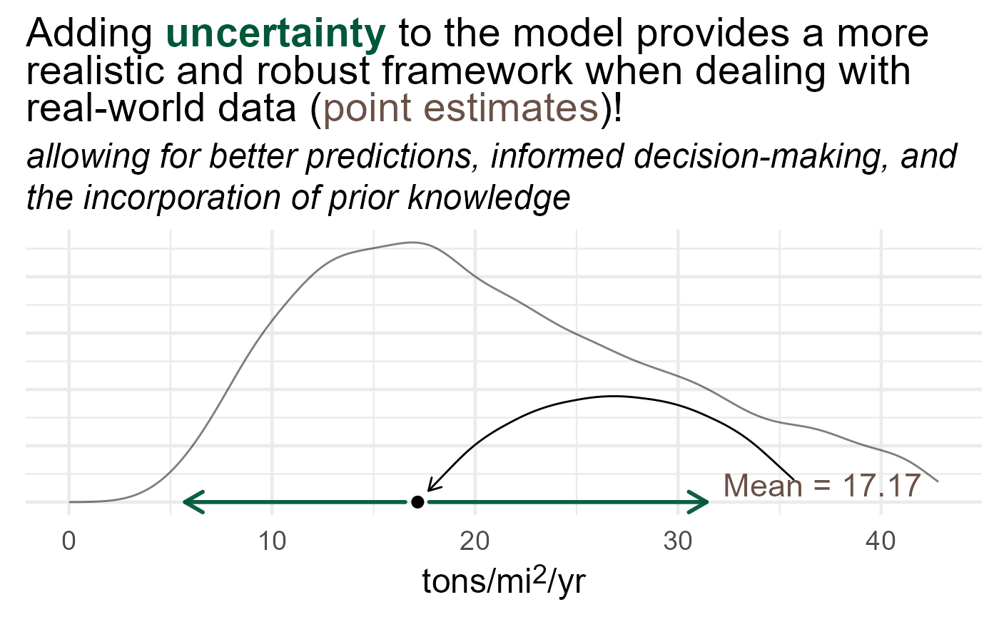
Figure 1
- Model
We want to model the response as a \(\text{Beta}\) distribution since it is bounded between 0 and 1. In addition, we modeled weak priors (high sigma) with both covariates (background erosion rates and GRAIP-lite specific area erosion rates) to account for the uncertainty associated \(\beta\) since we really have no prior knowledge of this relationship (\(Y \sim\beta_i\))
\[ Y_i \sim \text{Beta}(\mu_i, \phi) \\ \text{logit}(\mu_i) = \beta_0 + \beta_1\text{Natural} + \beta_2\text{Roads} + \beta_3\text{Geology} \\ \beta_0=\text{Normal}(0,1) \\ \beta_1,\beta_2=\text{Normal}(0,2) \\ \beta_3=\text{uniform}(0,1) \\ \phi = \text{Gamma}(0.01, 0.01) \]
- Posterior Predictive
Once we fit the model, we can then sample from the posterior to get a posterior predictive distribution.
Build Uncertainty
First, we need to get an idea of how we could add uncertainty to our sediment indicator. One way to do this is look for other data (graphs, tables, expert opinion, etc) and model a theoretical distribution from said data sources. This approach has it’s caveats for sure (bias, uninformed, non-causal relationships) but is much more robust than just taking a point estimate with no uncertainty when done responsibly. Based on domain knowledge, we are assuming two dominant geologic types: granitic and sedimentary. We understand that there is going to be a loss of heterogeneity in our stratification but hope that our adjusted model uncertainty can lessen this error. To infer background erosion rates we took data from Kirchner et al. (2001) and a reference to a sedimentary erosion rate from the Idaho DEQ TMDL for the North Fork CDA. This data was used as a starting point from which uncertainty was applied. Kirchner data was for granitic parent material and Idaho DEQ was for sedimentary parent material.
Granitic
The Kirchner data provides us with more than just a single specific area erosion rate. We took short-term rates (10-28 years) within 2.5-300 sq.km’s drainage areas within forested catchments as our empirical data. From these data, we then used the lognormal distribution as our theoretical basis. Reasons to use the lognormal distribution were due to the relatively thin tail towards zero and modest tailedness to the right of the central tendency. As you can see in Figure 2 below, we modeled the empirical data with a theoretical one where the central tendency (23.248) and variation (3.875) came from the left panel graph in Figure 2.
Sedimentary
The belt group coefficients were taken from the Idaho DEQ TMDL. This needs more work but ultimately works out to be around 5,155 kg/km2/yr with no inferred variance so we just assume a similar variance to the granitics, not perfect but going with the idea that we are likely wrong (error building). Below we converted the ton/acre/year in the left graph to kg/km2/year to get a lognormal distribution like the granitics. The same rationale for a lognormal in the grantics applied for the sedimentary group as well.
GRAIP-Lite
GRAIP-Lite uses a similar method to categorize the baserate by
geologic parent material. With that comes empirical data as well (see
below). In this analysis we used 21 kg/yr/m for granitics and 14 kg/yr/m
for sedimentary. We then converted the specific sediment delivered by
area (specdelFS_HA) from the WCATT national model run by
appropriate geologic base rates. In addition, we added error to the
modeled specdelFS_HA values based on accumulated road
length. This is due to the error decreasing as you accumulate more roads
when compared to GRAIP. Once this was done, we then had a empirical
distribution of specific sediment delivered by area in western Montana
within USDA-Forest Service administration lands.
Model
Geology
We need to account for granitic and sedimentary parent material so somehow we need to figure out the most dominant one in the HUC. We do this by intersecting coarse geology map by parent material and then for each HUC take the one with the highest proportion. From there we consider a HUC ‘granitic’ or ‘sedimentary’ based on this crude method.
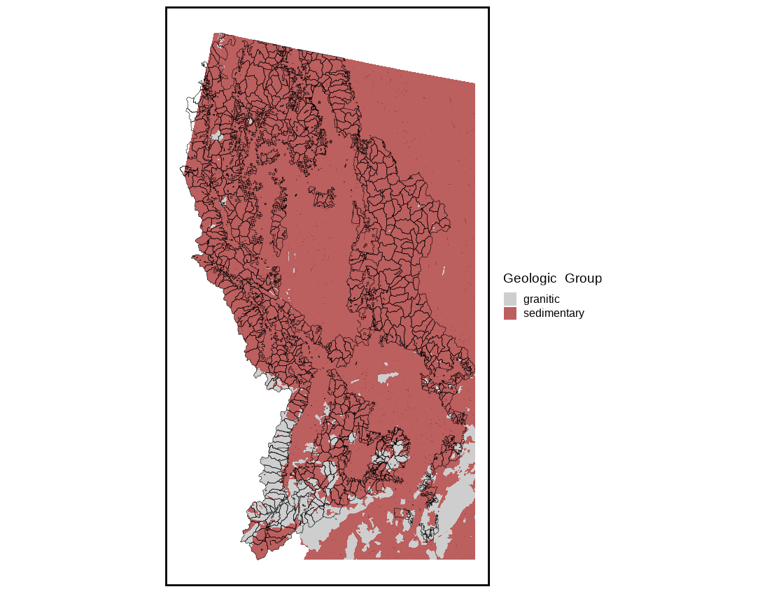
Figure 5
Bayesian Model
With all of the pre-processing done we can start to build the model. We went with a Bayesian model for a couple reasons; 1). the Bayesian model is able to provide a distribution of the likelihoods which can then be used as probabilities (great for Bayesian network), 2). being able to add weak or uninformative priors to the model parameters (betas, intercept, etc) helps with the inherent uncertainty and limits model overfitting.
To do this we need to use the data we generated prior and build up a faux model with uncertainty (Figure 6 light blue lines \(y_\text{rep}\)) so we can then take our empirical estimates (Figure 6 dark blue line \(y\)) to predict. When we predict with the empirical estimates, it will then give us that uncertainty that we built into the model.
Here is the model below in the code chunk. We just take our data generated from Figure 2, 3, and 4 compute the proportion and then model. Essentially what we are doing is sampling from inferred distributions, calculating a proportion, and then repeating. We can do this since our data is split by geologic group and when that happens our data is now exchangeable, meaning we can have a low road erosion with a low base erosion and vice versa. This is great because we can then theoretically sample as many events as we’d like!
priors.weak <- c(prior(normal(0, 1),class = 'b', coef = 'spec_delFS'),
                   prior(normal(0, 1), class = 'b', coef = 'base_erosion'),
                   prior(normal(0,1), class = 'Intercept')
                 )
sed_mod <- brm(
  proportion ~ spec_delFS + base_erosion + ig_or_not,
  family = Beta(),
  prior = priors.weak,
  data = sed_sim_filt)
)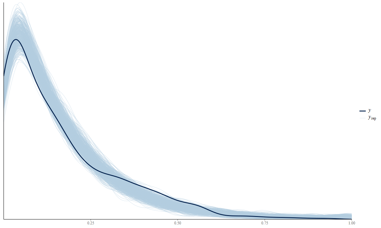
Figure 6
Posterior Predictive
Now that we built the model we can now use it on the empirical data we set out to use in the first place! All we do is predict with the model and then we get back a posterior predictive distribution. I won’t go into any more detail as it’s beyond the scope of this report but just know that the likelihoods generated from the model parameters with priors and sampling (MCMC) can shortcut complicated calculus to give us a probability distribution (see below)!
Below, is a few PP distributions with some of the empirical data. You can see how now we can get a range of probabilities and depending on the rating (FA, FAR, FUR) demarcation we can now add this information to the Bayesian network to help us with some decision making.
References
Kirchner, James W., et al. “Mountain erosion over 10 yr, 10 ky, and 10 my time scales.” Geology 29.7 (2001): 591-594.